Pre-print a cura degli autori. Originale pubblicato su:

NUCLEAR INSTRUMENTS AND METHODS 165 (1979) 325-332; © NORTH-HOLLAND PUBLISHING CO.

DEAD TIME CORRECTIONS IN COINCIDENCE MEASUREMENTS BY TIME-TO-PULSE-HEIGHT CONVERTERS OR STANDARD COINCIDENCE SYSTEMS

G. Faraci, S. Notarrigo and A. R. Pennisi

Istituto di Fisica dell’Università di Catania,

Gruppo Nazionale di Struttura della Materia del CNR, Catania,

Istituto Nazionale di Fisica Nucleare, Sezione di Catania, Italy

Received 7 March 1979

A definite probabilistic model for a time-to-pulse-height converter is studied taking into account dead time effects. Formulae are given for the time spectra and the coincidence rate. Two models for standard coincidence systems are also studied considering dead time either of the prolonging or non-prolonging type. All the theoretical models have been checked by Monte Carlo simulation.

1. Introduction

In many physical experiments either time‑to‑pulse‑height converters (TPHC) or standard coincidence systems (SCS) are employed in order to extract useful information related to the intensity of the coincidences or to the time distributions of correlated physical events.

In order to improve on the statistical accuracy it is often necessary to increase the intensity of the source of the physical events beyond the limits where effects connected with the finite time resolution of the apparatus can no longer be neglected^{1 ,2}).

The main effects connected with high intensities are dead time losses and pile-up distortions.

In such cases it is necessary to correct for such disturbing effects by the help of an exact theory developed for a realistic probabilistic model of the experiment.

In this paper we develop such theories for some models of TPHC and SCS.

2. Theory of the TPHC

2.1. general considerations

To be definite we shall consider a probabilistic model for the TPHC, having in mind the combination of the TPHC Ortec Model 467 together with the Gate and Delay Generator Ortec model 416A (GDG).

We consider trains of electrical pulses of negligible duration and with exponential distributions in two separate channels.

We assume that the pulses on the first channel act directly on the start input of the TPHC, while the pulses on the second channel act on the stop input of the TPHC after being delayed by the GDG.

Start-to-stop conversion is accomplished only after a valid start has been identified and after a stop pulse has arrived within the selected time range R.

The start input is disabled during the busy interval to prohibit pile-up; this introduces a dead time in the start channel equal to ξ + τ_ξ ; here ξ is either the time interval between the arrivals of the start and the stop pulses in case of an effective conversion or the range R in case of an out-of-range conversion, i.e. if no stop pulse arrived within the time range. τ_ξ  is an additional dead time different in the two cases, namely

Also the GDG input is disabled for a constant time interval τ after eaeh passed stop pulse.

Because of the dead times introduced by the TPHC and the GDG the actual distributions of the interarrival times of the pulses in the two channels will no longer be exponential, however the new distributions can be easily deduced.

We shall be mainly interested in the time spectrum, i.e. in the distributions of the time intervals between a valid start and the first stop pulse.

2.2. accidental coincidences

We first consider only the time spectrum of the accidental coincidences, i.e. assume that the distributions of the interarrival times of the pulses in the two channels are independent.

The two previously named cases (a) and (b) will be treated separately.

Referring to fig. 1, let us first consider case (a) and let X, Y_k, W, Z be random variables representing respectively:

- the time length of the previous conversion process,

- the interarrival time between two effective consecutive pulses in the stop channel,

- the waiting time for the first start pulse following the instant in which the start input circuit of the TPHC is again free to accept pulses after the preceding conversion,

- the time interval between the instant in which the GDG is again free to accept other incoming stop pulses, after the last stop pulse arrived before start, and the instant in which the next stop pulse has arrived to complete the conversion process.

We adhere to the methods and the terminology of the renewal theory as expounded in ref. 3.

We look for the probability H_ξ (x) of having a conversion with time length less than x given that the preceding conversion had length X = ξ  (ξ < R).

This event occurs if a start pulse arrives with W = w, m effective pulses have arrived in the stop channel following the stop pulse of the preceding conversion and before the new start pulse, i.e.

U_m = Y₁+Y₂+...+Y_m = u , (u < τ₁ + w),

and finally the next pulse on the stop channel arrives with Z = z and

(τ₁ + w) - (u + τ) £ z £  (τ₁ + w) - (u + τ) + x .

All this for some possible combinations w, u, z, m .

If g₁(αw), h_m(βu), g₁(βz) are, respectively, the probability densities for W, U_m, Z, we have, summing over all possible m and integrating over all possible w, u, z

(1)

It remains to write down the expression for the probability densities:

- for W and Z, given the hypothesis of our model

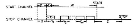
Fig. 1. Schematical diagram of the pulse sequence in the two channels of the TPHC.

(exponential distribution for the incoming pulses on both channels), we can write

g₁(αw) º α e^{- α w} , (w ³ 0) ;

g₁(βz) º β e^{- β z} , (z ³ 0) ,

with α and β the incoming intensities in the start and stop channel respectively and g₁ (x) º 0 for x < 0;

- for U_m we must write the convolution integral of m independent arrivals taking into account the dead time of GDG; this can be done by introducing the random variables V_k, with a common exponential distribution representing the interarrivai times of the incoming pulses at the GDG input.

Remembering that the Y_k represent the interarrival times of the effective pulses on the stop input after leaving the GDG, which remains blocked during an interval τ after each effective pulse has been passed on, we can write³)

Y_k = V_k + τ .

After performing the convolution integrals we have

h_m(βu) º g_m [β (u - m τ )] , (u > m τ , m³ 1) ,

h_m(βu) º 0 , (u £ m τ , m³ 1).

Here

is the derivative of the modifìed incomplete gamma function⁴’⁵), namely

.

We note that the summation in eq. (1) is extended to m = 0 to take into account the possibility of having a stop pulse after start without any previous pulse in the stop channel between the preceding conversion and the new start pulse, by assuming an atom of unit weight at the origin, i.e. h₀(βu) º δ(u) ³).

The infinite sum and the integrals in eq. (1) can be easily performed by the properties of the incomplete gamma functions⁴’⁵), we do not give here the lengthy formal manipuiations.

The final result is

(2)

where

,

,

τ_m º τ₁ - (m+1)τ ,

M º integral value of the ratio τ₁/τ.

G_m+1(x) are the modified incomplete gamma functions previously introduced with the convention

G_m+1(x) º 0 for any x £ 0.

In case (b) (ξ = R) we may consider a delayed renewal process³) by redefining:

U_m = U₀ +Y₁+Y₂+...+Y_m ;

under the hypothesis τ < R (this can practically always be achieved), U₀ has a probability density given by and, in such case, it can be easily demonstrated that H_ξ=R (x) will be formally identical to H_ξ=R (x) as given by eq. (2) after the formal substitution

.

In order to find out the distribution independently of the length of the preceding conversion we note that H_ξ (x) can be regarded as the transition probability of a simple Markov process as defined in ref. 6 and because it depends on ξ only through τ_i^*(i=1 for ξ < R, i=2 for ξ = R), the Chapman‑Kolmogorov equation, valid for any Markov process^3,6) reduces in this case to the Bayesian formula

(3) H(x) @ H(R)×H_ξ<R (x) + [1 - H(R)] H_ξ=R (x).

This also because it can be demonstrated by the properties of the incomplete gamma functions, that H_ξ (x) is a non-defective probability distribution [i.e. H_ξ (¥)= 1].

H(R) can be easily determined by putting x = R in formula (3) and fìnally we may write

(4)

which expresses the time distribution of the accidental coincidences in our model of TPHC in terms of the conditional probability distributions H_ξ (x) previously derived in the two cases (a) and (b).

2.3. correlated events

Of course before studying the effect of correlated events in the two channels we must postulate a specific conditional probability distribution of having a pulse in the stop channel at time t′ given a pulse on the start channel at time t.

We assume that this distribution admits a density which we indicate by ρ_t (t′).

We first consider the limit case

(5) ρ_t (t′) = δ(t′ - t + r) ,

with δ(x) the Dirac function.

However we shall assume also uncorrelated pulses arriving with an intensity α - γ in the first channel and β - γ in the second channel, γ being the intensity of the correlated events.

So four different possibilities must be considered:

1) The start pulse has no correlated event in the stop channel, and will give an accidental coincidence with any pulse in the stop channel (either of the correlated stock or else) arriving within the time range.

2) The start pulse has a correlated event in the stop channel delayed by r [according to eq. (5)], however the true coincidence will be lost because of the arrival of any other pulse before the arrival of the correlated one.

3) The start pulse has a correlated event in the stop channel but the true coincidence will be lost by the dead time of the GDG, so an accidental coincidence will result by the arrival of any other pulse within the time range.

4) The start pulse has a correlated event on the stop channel; events under (2) or (3) do not occur, so we have a true coincidence.

Before proceeding to the derivation of the relevant formulae it must be pointed out that in this case of correlated events the conditional probability may not in general have the simple Markov property (as defined in ref. 6), because the probability distribution of the waiting time for the first stop pulse after start depends on the probability distribution of the incoming pulses in the stop channel which in turn, because of the delayed correlation, depends on the previous occurrence of the correlated pulse in the start channel and, because of the dead time of the anti-pile-up blocking circuit of the start input, on the preceding history of the process.

However, if the intensity ratio of the correlated events is small as compared to the total intensity in the stop channel (γ / β << 1) the process will be approximately simple Markov, because we do not have to worry, in this case, about the detailed distribution of the correlated events in the stop channel.

In such an hypothesis we can write for the conditional probability distribution of the waiting time of an effective stop pulse after a valid start, given a preceding conversion length ξ.

(6)

with

the contribution of process (1).

the contribution of process (2),

the contribution of process (3),

the contribution of process (4),

and

(7)

(8)

is obviously identical to the integral appearing in formula (1) and can be expressed by the right hand side of formula (2).

The right hand side of formula (8) may be integrated by the same methods and gives

(9)

[obviously if r > τ or x < r],

here the function is given by the right hand side of formula (2) with, however, M º integral value of the ratio (τ₁ + r) / τ and

(10) ,

with

and the other quantities as previously defined.

Obviously also in this case the a priori probability can be obtained by formula (4).

In the more general case of an arbitrary density ρ_t′ (t), to find out the general formulae we can derive the distribution function for the limit densities eq. (5), , and use this as the Green function of a randomized process³), i.e.

(11)

We have here made the usual assumption of translational invariance:

ρ_t (t′) = ρ (r) , r = t′ - t.

Also in this case the a priori probability distribution will be given by formula (4) in terms of the a posteriori probabilities given by eq. (11) for the two cases (a) and (b) after the usual sobstitution .

2.4. monte carlo simulation

In order to get some insight in the more general case we have simulated our TPHC model by a Monte Carlo method.

This allowed us also to check all previously derived formulae.

The model consists in generating, by standard method, the interarrival times in the two channels with initial exponential distribution and checking the eventual losses for dead time.

In figs. 2 and 3 the comparison of the Monte Carlo results with the exact formulae previously derived is shown. The theoretical curves given by formulae (2) and (4) are normalized to the relative Monte Carlo results by their respective maximum values.

The Monte Carlo curves were computed by their absolute values, but in the figures they are normalized to the linear approximation, in order to give an idea of the dead time losses (i.e. the ordinate H / H₀ represents the ratio of the effective coincidence rate to the product αβtR/100, where t is the counting time).

The agreement is very good within the statistical error introduced by the Monte Carlo computations: this statistical error, even if not signifted in the

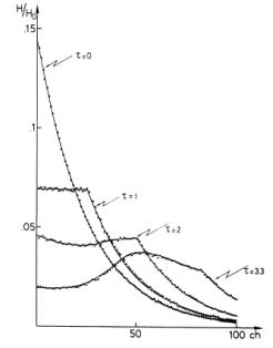
Fig. 2. Time spectra of the TPHC according to the exact formulae derived for the accidental coincidences (continuous lines) compared with the results of the Monte Carlo simulation (points). The theoretical curves are normalized at the maximum value to the respective Monte Carlo calculations. The Monte Carlo curves are normalized to the linear approximation (see text) in order to show the dead time losses. Fixed parameters: α = β = 1 μs^-1 , τ₁ = 5 μs, τ₂ = 4 μs, R = 4 μs. Varying parameter: τ = 0, 1, 2, 3.3 μs. See text for the meaning of the parameters.

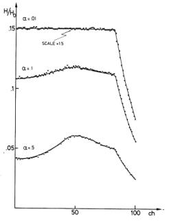
Fig. 3. Same as fig. 2. Fixed parameters: β = 1 μs^-1 , τ₁ = 5 μs, τ₂ = 4 μs, τ = 3.3 μs, R = 4 μs. Varying parameter: α = 0.01, 0.1, 0.5 μs^-1 . The ordinate value for α = 0.01 should be multiplied by a factor 1.5.

figure, can be estimated by the scattering of the points around the theoretical curves.

In figs. 4 and 5 the approximate formulae for processes, not simple-Markov, as given by formulae (4), (7) and (8), are compared with the Monte Carlo computations.

We note that for accidental coincidences with low intensities in the start channel the interarrival times between consecutive and effective start pulses will be long enough and if ατ << 1 the distribution of the interarrival times on the stop channel may be considered as stationary, in this case we know that because of the renewal theorem applied to persistent renewal processes³), the distribution of the residual waiting time can be expressed in terms of the distribution of the interarrival times on the stop channel by³)

,

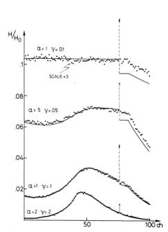
Fig. 4. Same as fig. 2 for the approximated formulae derived in case of partially correlated events. Fixed parameters: τ₁ = 5 μs, τ₂ = 4 μs, τ = 3.3 μs, r = 3 μs, R = 4 μs, γ/α = 0.1. Varying parameter: α = β = 0.l, 0.5, 1, 2 μs^-1 . The ordinate value for α = β = 0.l μs^-1 should be multiplied by a factor 3.

and, because in our case

we obtain

If we also have βR << 1 we get the often quoted linear approximation

H(x) = βx , for any x < R.

The validity of these approximations can be checked in fig. 2.

As a final point we note that the renewal theorem can be used to obtain the coincidence rate for the limit distribution eq. (5). In fact we may consider

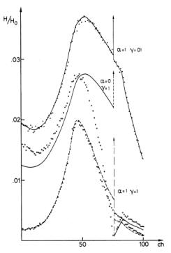
Fig. 5. Same as fig. 4. Fixed parameters: τ₁ = 5 μs, τ₂ = 4 μs, τ = 3.3 μs, r = 3 μs, R = 4 μs. Varying parameters: α = β = l μs^-1 and γ = 0.1, l μs^-1 ; α = β = 0 μs^-1 and γ = l μs^-1

the process originated by the random variable

and apply the renewal theorem to the number of renewal epochs³). So we may affirm that the number of effective start pulses in a long counting interval t is approximately normally distributed³) with expectation t / μ and variance tσ² / μ³, where

,

and ;

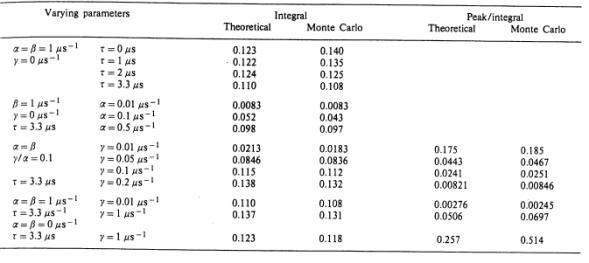
TABLE 1

Coincidence rate per μs, integrated over the entire time range of the converter and ratio of the number of the events under the peak and the integral spectrum. Fixed parameters (see text): τ₁ = 5 μs, τ₂ = 4 μs, r = 3 μs, R = 4 μs.

In practical calculations for μ we have used the approximate formula

(12)

Here .

In the stationary approximation the measured true coincidence rate obtained after subtraction of the accidental coincidence rate is given by

.

This last formula allows to correct in a simple way for dead time losses whenever the linear approximation is justified.

In table 1 the absolute value given by the approximated formula (12) is compared with the Monte Carlo computation. A comparison of the peak-to-integral ratio between the model and the Monte Carlo simulation is also shown in table 1, as deduced by the spectra. This ratio is independent of the approximations of formula (12) and so gives an idea of the error introduced by the non-Markovian character of the process.

3. Standard coincidence system

3.1. dead time of the non-prolonging type

We here consider trains of electrical pulses of negligible duration and with exponential distribution in two separate channels as before. However, the pulses act on two time pick-up units which generate pulses of duration τ₁ in channel one and τ₂ in channel two.

The two time pick-up units remain blocked for a time equal to the duration of the output pulses. This introduces in the two channels dead times of the non-prolonging type⁷).

The effective pulses coming out of the two time pick-up units will be processed by the coincidence circuit which will give an output pulse whenever an effective pulse arrives in channel one (two) during a time interval equal to the duration of the pulse in channel two (one) starting from the arrival of a pulse in channel two (one), plus the symmetrical case.

In the absence of correlated pulses in the two channels, by the often quoted renewal theorem³’⁶) the distribution of the waiting time of a pulse in the second channel after the arrival of a pulse in the first channel can be considered as stationary, for sufficiently long counting times, so that the accidental coincidence rate will be given by the product of the expectation for the number of pulses in one channel during the counting time t, by the expectation for the number of pulses in the other channel during a period τ₁ + τ₂, in the stationary approximation, i.e.

(13) ,

α and β being the intensities of the pulses in the two channels before the time pick-up units.

In case we have correlated pulses in the two channels with intensity γ, we note that such pulses will always be counted without dead time losses, unless the preceding pulse blocking the time pickup unit with shorter dead time is also of the correlated stock.

This is because any correlated pulse which arrives within the dead time originated by a preceding pulse of the non-correlated stock, to the effect of the coincidence output will be replaced by the killing pulse, so that, if τ₁ £ τ₂, the total (i.e. true plus random) rate will be

(14)

If, as usual, the random coincidences are measured only partly by inserting a convenient delay in one channel, the intensity γ can be deduced by formulae (13) and (14) by measuring independently, besides n_A and n_T, the intensities α and β and the ratio τ₁ / τ₂.

If γ << α and γ << β we obviously have for the true coincidence rate

.

3.2. dead time of the prolonging type

The case in which the time pick-up units prolong the output high voltage level, when another pulse arrives during an interval of time equal to the processing time for a single pulse, has already been considered by other authors⁷’⁸).

However, the formulae they give are not correct, in fact one formula gives wrong results for higher incoming intensities⁸), the other for longer resolving times⁷).

In order to get the correct formula for the random coincidence rate we observe that if in channel one (two) arrives a pulse able to pass through the time pick-up unit [i.e. no previous pulse has arrived in a time interval τ₁ (τ₂) before it], then any pulse whatever arriving in channel two (one) in a time interval τ₂ (τ₁) before it, will produce an accidental coincidence. So the accidental coincidence rate will be given by the product of the number of pulses arriving in channel one (two), during the counting time t by the probability of having no other pulse in the same channel within a interval τ₁ (τ₂) before the instant of arrival of the pulse which originates the coincidence, by the probability of having a pulse in channel two (one) within an interval τ₂ (τ₁) before it, plus the symmetrical case, i.e.

(15)

In case of correlated pulses in the two channels with intensity γ by the same considerations made in sect. 3.1 we have for the total coincidence rate (τ₁ < τ₂)

(16)

We note that formulae (13) – (16) can be generalized to the case of an n-fold coincidence system by the methods considered in refs. 7, 8.

Formulae (13) – (16) have also been checked by Monte-Carlo simulation with an accuracy better than 1%.

We thank Prof. V. I. Goldanskii for useful discussions.

References

1) J. Radeloff, N. Buttler, W. Kesternich and E. Bodenstedt, Nucl. Instr. and Meth. 47 (1967) 109.

2) J. Glatz, Nucl. Instr. and Meth. 79 (1970) 277.

3) W. Feller, Introduction to probability theory and its applications (J. Wiley, New York, 1971).

4) M. Abramovitz and I. A. Stegun, Handbook of mathematical functions (Dover Publ, New York, 1965).

5) A. Erdelyi, Higher transcendental functions (McGraw-Hill, New-York, 1953).

6) J. L. Doob, Stochastic processes (J. Wiley, New York, 1953).

7) V. I. Goldanskii, A. V. Kutsenko and M. I. Podgoretskii, Counting statistics of nuclear particles (Hindustan Publ. Co., Delhi, 1962).

8) L. I. Schiff, Phys. Rev. 50 (1936) 88.